Information Transfer Rate: The Engineering Metric That Should Drive Your BCI Design Decisions

Information Transfer Rate (ITR) is one of those metrics that separates researchers who build BCI systems from those who deploy them. Accuracy tells you how often your decoder is right. ITR tells you how fast it communicates. These are not the same thing — and the gap between them determines whether a system is clinically useful or just academically interesting.

This post explains the ITR formula from the ground up, walks through what it means for your pipeline architecture, and shows how to compute it directly with the Nimbus Python SDK — the same deploy loop you’d use when you take a model from calibration into live inference (From Training to Streaming: Deploying a Live EEG Decoder with the Nimbus Python SDK).

What Is Information Transfer Rate?

ITR measures how many bits of information a BCI system can transmit per unit time — typically expressed in bits per minute. It was formalized by Wolpaw et al. (2000) and remains the standard benchmark for comparing BCI paradigms across labs.

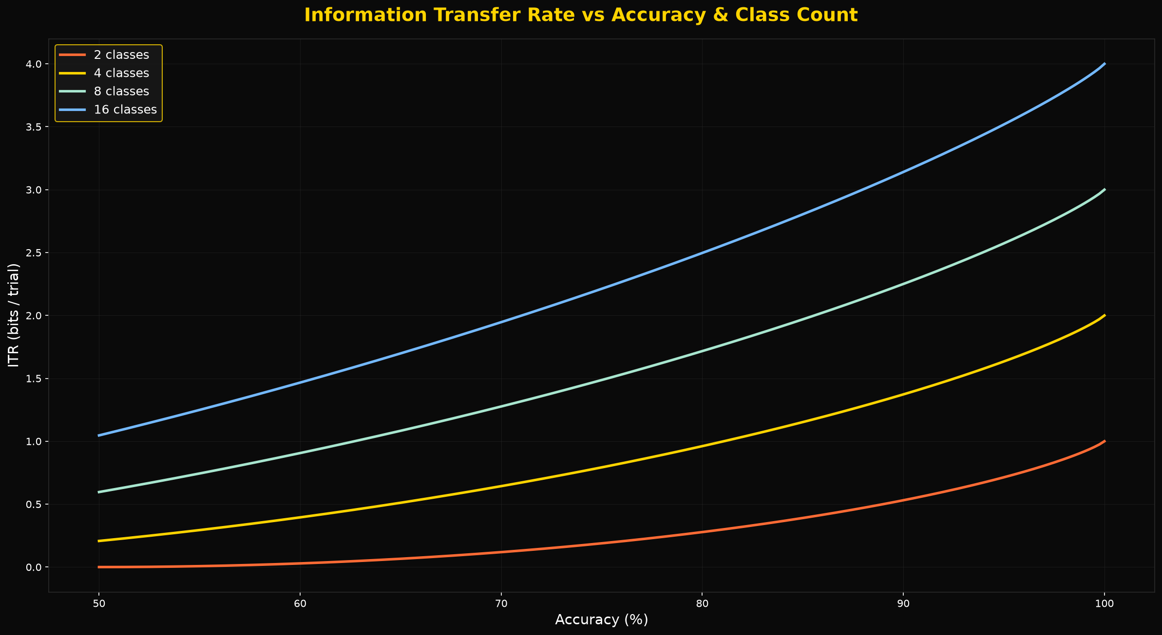
The formula has two parts. First, the information transferred per trial (B, in bits):

• If accuracy p equals chance (1/N for N classes): B = 0
• If accuracy p = 1.0: B = log₂(N)
• Otherwise: B = log₂(N) + p·log₂(p) + (1−p)·log₂((1−p)/(N−1))

Second, ITR per unit time:

ITR (bits/min) = B / trial_duration × 60

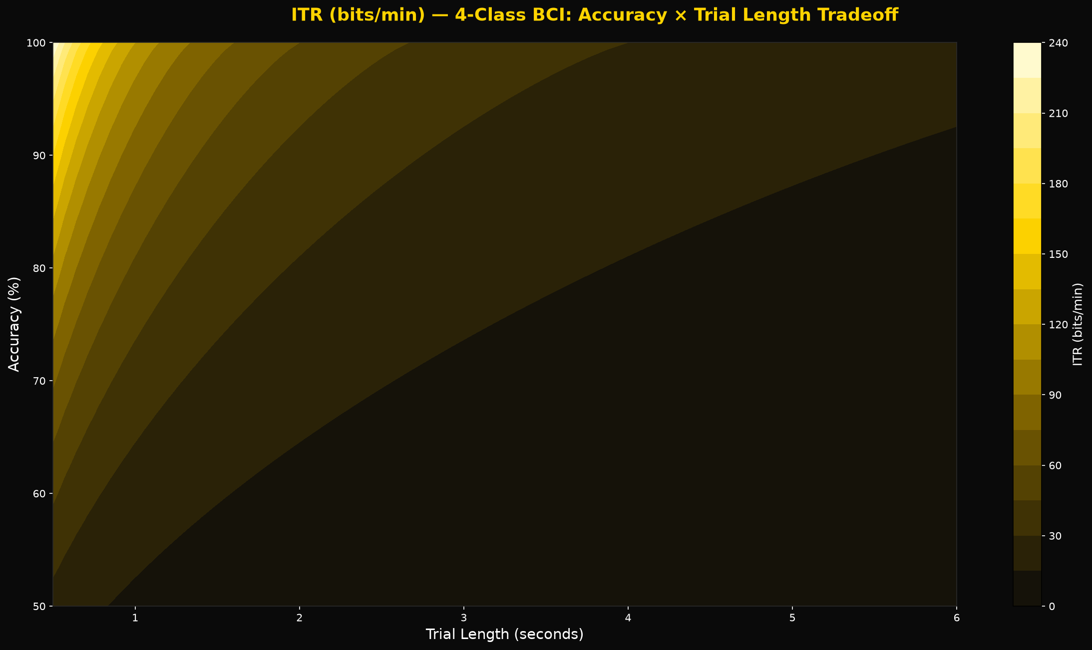
This compound structure is what makes ITR so useful: it forces you to confront the tradeoff between accuracy and speed. A system that takes 8 seconds per trial at 95% accuracy can underperform one that takes 2 seconds at 80%, depending on class count.

Why Accuracy Alone Misleads You

Optimizing a BCI decoder purely for accuracy creates a perverse incentive: you can always raise accuracy by using longer trial windows, heavier preprocessing, or more conservative rejection policies — all of which increase latency and reduce throughput.

Consider two motor imagery decoders, both 4-class:

• Decoder A: 93% accuracy, 5-second trial → B ≈ 1.62 bits → ITR ≈ 19 bits/min
• Decoder B: 82% accuracy, 2-second trial → B ≈ 1.18 bits → ITR ≈ 35 bits/min

Decoder B communicates nearly twice as fast despite appearing weaker on the accuracy scoreboard. This is not a pathological example — it is the typical regime for deployed BCI systems, where communication speed matters as much as correctness.

The implication for Nimbus Studio pipelines is concrete: when comparing two pipeline variants, always include ITR alongside accuracy in your results_output node. Accuracy without ITR is an incomplete benchmark — and for real deployments it pairs naturally with confidence gating, where you trade off coverage vs. correctness to maximize useful throughput (Confidence-Gated BCI: How Entropy and Rejection Policies Keep Decoders Reliable in the Real World).

The Class Count Dimension

ITR increases with class count — but only when accuracy holds up. Adding more classes raises the theoretical ceiling (log₂(N)) while compressing the margin for error.

For most BCI paradigms, this creates a practical sweet spot:

• SSVEP (CCA node): High ITR because CCA extracts strong frequency-locked features that scale well with class count. 4–16 classes at 60–90% accuracy routinely exceeds 50 bits/min.
• P300 (xDAWN + Nimbus LDA): Moderate ITR. The class count is effectively the speller vocabulary size, but accuracy degrades with noisy ERP signals and low trial counts.
• Motor Imagery (CSP + Nimbus LDA or Nimbus Softmax): Lower ITR because trial durations are longer and class counts rarely exceed 4 in practice.
• Hybrid pipelines (FBCSP + Nimbus STS): Can recover ITR by adapting trial timing online as the decoder's posterior uncertainty stabilizes.

Computing ITR with the Nimbus Python SDK

The Nimbus Python SDK's nimbus_bci.metrics module includes an ITR calculator that handles edge cases (accuracy at or below chance, single-trial inference) and integrates with the BatchResult returned by predict_batch.

from nimbus_bci.metrics import information_transfer_rate

# BatchResult from predict_batch includes per-trial accuracy and confidence
result = classifier.predict_batch(X_eval, trial_duration_s=2.5)

itr = information_transfer_rate(
    accuracy=result.accuracy,
    n_classes=4,
    trial_duration_s=2.5,
)
print(f"ITR: {itr:.1f} bits/min")

For streaming pipelines, you can track rolling ITR over a sliding window of recent trials — letting you detect session-level drift before it becomes a user-facing problem.

The evaluate_rejection_policy function is a natural companion. When you gate predictions on Bayesian confidence (via entropy thresholds from the SDK), effective ITR can actually increase: rejected trials reduce throughput but protect accuracy on answered trials more than proportionally, especially when rejections cluster on the noisiest or most ambiguous epochs. The right rejection threshold is the one that maximizes ITR, not the one that maximizes accuracy on accepted trials (see Confidence-Gated BCI: How Entropy and Rejection Policies Keep Decoders Reliable in the Real World).

Connecting ITR to Nimbus Studio Pipeline Decisions

ITR translates directly into the design choices you make in Nimbus Studio:

Trial duration (Epoching node): Shorter epochs raise ITR when accuracy holds. Use cross_validation to sweep trial lengths and plot ITR at each setting rather than just accuracy. The optimal epoch for ITR is almost always shorter than the epoch that maximizes accuracy (more on setting those windows correctly in Epoch Design and Trial Structure in BCI: How Your Protocol Shapes Your Decoder).

Preprocessing depth: Heavy artifact removal (ICA, AutoReject via the Artifact Rejection node) improves accuracy but adds calibration overhead. For deploy pipelines, lighter preprocessing combined with a Signal Quality Monitor gate often achieves better ITR than a clean-but-slow preprocessing stack.

Class count (template design): More classes raises the ITR ceiling — up to the point where below-chance performance on any individual class collapses the composite metric. Use cross_validation per-class to identify which classes are dragging down overall ITR before committing to a paradigm.

Decision Policy node: In streaming deploy, temporal smoothing adds effective latency that directly cuts ITR. Tune the debounce window to the minimum that prevents unsafe output chatter — not the maximum that makes demos look stable.

Adaptive decoding (Nimbus STS): The rxsts_sdk node's latent-state dynamics can implicitly shorten effective trial duration by building certainty faster in high-SNR epochs. Monitor posterior entropy per trial: when entropy drops below threshold before the epoch ends, early-stopping the trial is a principled ITR optimization that can yield 15–30% throughput gains in favorable sessions.

Conclusion

Information Transfer Rate is not just an academic benchmark — it is the engineering constraint that makes the accuracy-speed tradeoff legible during development and defensible at deployment. A BCI that communicates faster under realistic conditions is more useful, even if it scores lower on a single accuracy number.

The Nimbus Python SDK makes ITR a first-class citizen of your evaluation loop. Nimbus Studio's pipeline architecture gives you the levers to optimize for it directly: trial duration, class count, rejection thresholds, and adaptive decoding all move the ITR needle in predictable, measurable ways. And once you’re treating uncertainty and throughput as co-equal constraints, you can also make calibration itself more data-efficient by selecting trials based on posterior uncertainty (Active Learning for BCI Calibration: How Bayesian Uncertainty Drives Smarter Trial Selection).

The next time you compare two pipeline variants, plot ITR alongside accuracy. You may find that the "worse" decoder is actually the better product.